1.5x faster MoE training with custom MXFP8 kernels
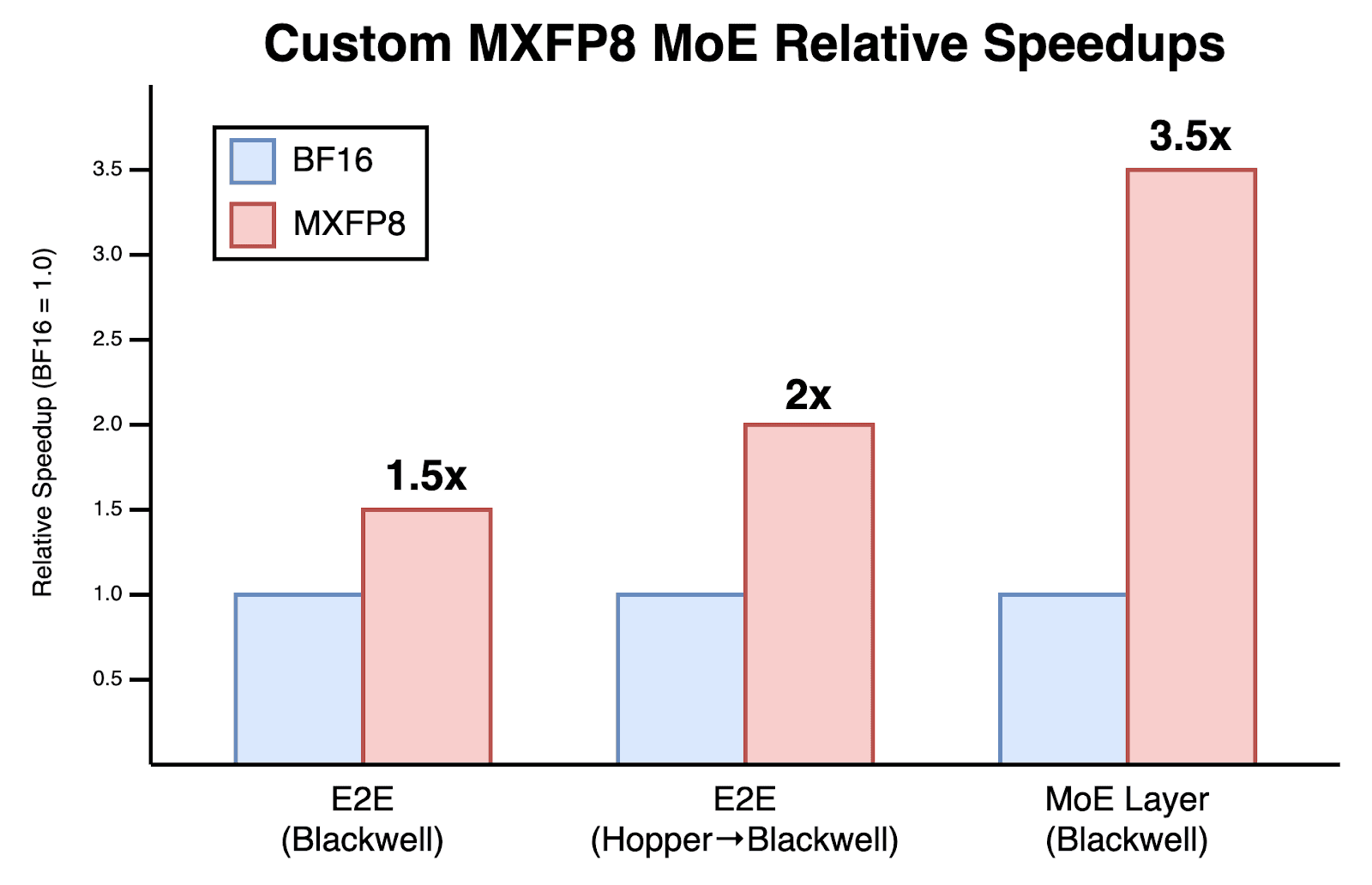
Achieving a 3.5x MoE layer speedup with a complete rebuild for Blackwell GPUs.
We want to build the world’s best AI coding models, but training large language models can be expensive. For instance, our largest internal models can take weeks to train on tens of thousands of GPUs. This is not only computationally expensive, but it also slows the pace at which improvements reach our users.
We recently began upgrading from Hopper GPUs (H100s) to Blackwell GPUs (B200s) and saw this as an opportunity to deeply optimize our training workloads. Profiling revealed that the main bottleneck was the Mixture-of-Experts (MoE) layer, implemented with MegaBlocks, which accounted for nearly 53% of forward-pass time and 27% of backward-pass time.
That’s why, over the past few weeks, we rewrote the entire MoE layer from scratch at the GPU kernel level with zero dependencies on any CUDA libraries. Instead, we used pure, good old CUDA and PTX, with a few bits of ThunderKittens sprinkled in. As a result, we achieved a 3.5x improvement in MoE layer performance for both the forward and backward passes, translating to a 1.5x end-to-end training speedup on Blackwell and a 2x speedup compared to our original Hopper setup. We believe our stack is faster than any combination of open-source alternatives available today.
Most of this improvement came from transitioning from BF16 to MXFP8 which we achieved with nearly zero loss in training quality. But this also taught us that going low precision is easier said than done. If not done carefully, MXFP8 training may offer minimal performance improvement over BF16 due to various kernel overheads. The MXFP8 training recipe is also not widely shared, meaning you have to discover the right approach yourself.
The following is our recipe, and a look at the ML work we do at Cursor.
A quick introduction to the Microscaling (MX) data formats
A common way to reduce the computational cost of large deep learning models is to use lower-precision activations and weights. However, converting them to narrow bit-width formats (e.g., 8 or fewer bits) introduces unacceptable rounding error unless the values are scaled appropriately. For example, some weights in a large model might be 0.0001, 0.0005, or –0.0007, but naively converting these to FP8 would round them all to the same number: zero, since the smallest positive value representable in FP8E4M3 is around 0.0019.
To address this, it is common to apply a per-tensor scaling factor, which rescales the tensor while keeping its values within the representable range of the target data format. This ensures that the available dynamic range is fully utilized. For example, if a tensor’s values are all between –0.0001 and 0.0001, its scaling factor could be set to 4,480,000. This would cause the tensor’s values after scaling to be in the range [–448, 448], which corresponds to the representable bounds of FP8E4M3.
Microscaling goes a step further by applying scaling to fine-grained sub-blocks of a tensor, rather than using a single scale factor for the entire tensor. The Microscaling (MX) format standardizes this approach by defining a set of low-precision, micro-scaled data formats. Full details are provided in its specification, which defines the following concrete MX-compliant formats:
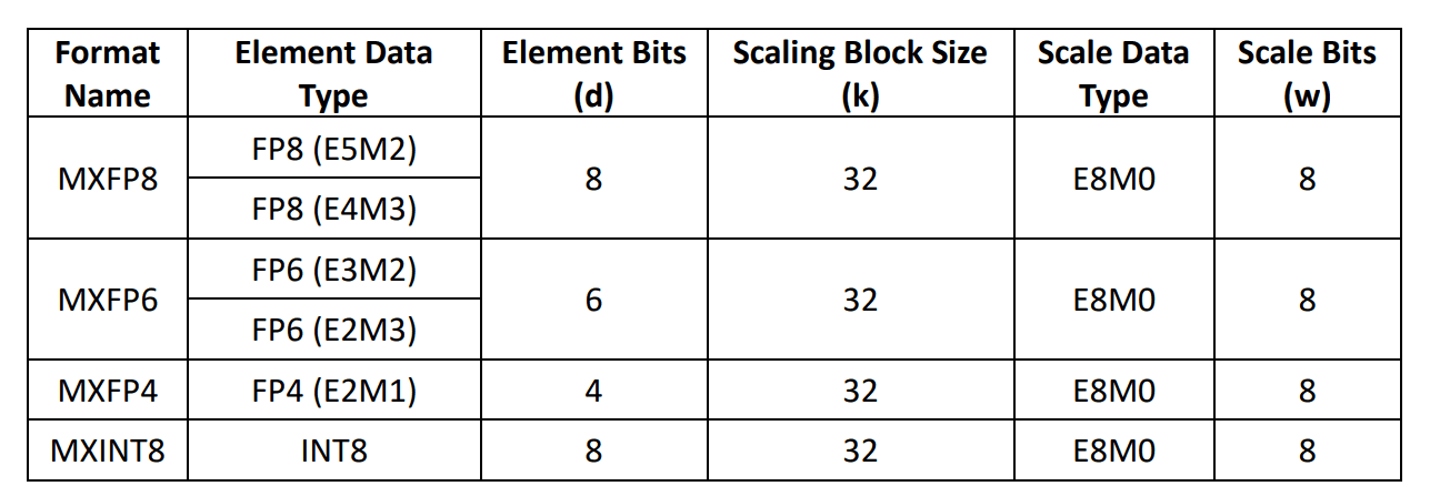
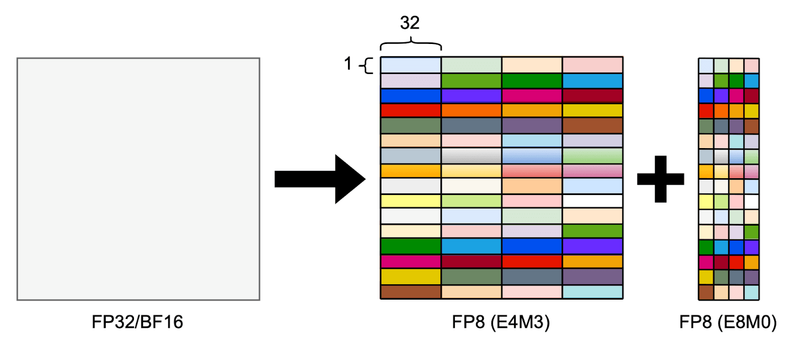
For example, if we use the MXFP8 format with the E4M3 element type, the data would consist of FP8E4M3 elements with an FP8E8M0 scale factor applied to every consecutive 32-element block, as illustrated in the figure below.
Although microscaling can unlock significant performance gains, applying it in practice introduces several challenges and depends heavily on the underlying hardware. Let’s first look at why applying microscaling on NVIDIA Blackwell GPUs can be particularly challenging.
1. Tensor memory and CUDA cores kill the dequantization vibe
In microscaled FP8 matrix multiplication, the computation is broken into smaller block-sized steps along the reduction dimension. After each blocked matrix multiplication, the partial result is dequantized using scale factors and then accumulated before proceeding to the next block.
For example, in the well-known DeepSeek V3 (DSV3) technical report, the A matrix was scaled in blocks of size and the B matrix was scaled in blocks of size . This means the procedure is as follows:
- Perform a 128-block matrix multiplication:
C_block = A[:, k*128:(k+1)*128] @ B[k*128:(k+1)*128, :]- Apply dequantization using scale factors:
C_block = A_scale[:, k] * C_block * B_scale[k, :]where A_scale is broadcast across 128 elements along the K dimension and B_scale is broadcast across 128 elements along both dimensions
- Accumulate the dequantized block:
C += C_block- Proceed to the next block along the reduction dimension:
k += 1This method naturally works well on the Hopper architecture (on which DSV3 was trained), because (1) the results of the tensor core matrix multiplies (via wgmma instruction) are accumulated in registers, and (2) you can pipeline matrix multiplies, asynchronously launching other tensor core matrix multiplies while performing dequantization with CUDA cores. Because everything is accumulated in the registers, no additional data movement is required between the matrix multiplies.
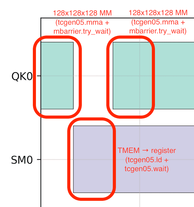
This is no longer the case on Blackwell GPUs due to tensor memory (TMEM). TMEM is a new set of on-chip, SM-local memory added on Blackwell GPUs. Unlike Hopper GPUs, where the results of tensor core matrix multiplies accumulate directly in registers, Blackwell GPUs accumulate them in TMEM (via tcgen05.mma instruction). To perform custom arithmetic on the accumulators, you must transfer the results from TMEM to registers, process them with CUDA cores, write them back to TMEM, and then wait for all of these instructions to complete because the data movements are asynchronous. Although TMEM is faster to access than shared memory (SMEM), this still kills tensor core occupancy.
At first glance, this suggests a pipelined approach: divide the TMEM into chunks and run matrix multiplies on one chunk while data movement and dequantization are happening on the other chunk.
But there’s another problem here: while the Blackwell tensor cores doubled in TFLOP/s compared to Hopper, the FP32 CUDA cores only improved by about 33% (60 → 80 TFLOP/s). With 32-block scaling, the amount of computation spent on dequantization is 1/32 the matrix multiply (both involve multiplication and addition; with CUDA core dequantization you have to manually accumulate), but the speed of dequantization is 1/56 the matrix multiply (4,500 TFLOP/s theoretical). As a result, dequantization on CUDA cores can take nearly 1.76x the time spent on matrix multiplication. This is horrible.
| Hopper (H100 SXM5) | Blackwell (B200) | |
|---|---|---|
| FP8 Tensor Core Throughput | 1,979 TFLOP/s | 4,500 TFLOP/s |
| FP32 CUDA Core Throughput | 60 TFLOP/s | 80 TFLOP/s |
| 32-Block Dequantization Time (relative to matrix multiply) | 1.03x | 1.76x |
Table 2. Relative Dequantization Cost on Hopper vs Blackwell.
Empirically, we could not even surpass Hopper’s realistic FP8 throughput of 1,500 TFLOP/s with any variation of the above approach. And this isn’t even considering the quantization overhead.
2. Death by a thousand quantizations
Every matrix has to be FP8-quantized before getting fed to a FP8 matrix multiplication kernel. It’s essential to reduce and hide the quantization time as much as possible. When not handled carefully, quantization kernels can overtake the GPU time.
To understand how dominant quantization can be, let’s consider a simple matrix multiplication , where:
-
is
-
is
-
is
In grouped matrix multiplications for MoE training, it’s common for to be very large compared to and . So let’s take:
With this, the total number of floating point operations needed for the matrix multiplication itself is:
Our benchmarks show that Blackwell GPUs (B200s) have an FP8 matrix multiplication throughput of ~3,300 TFLOP/s. This means the expected wall-clock time to execute the matrix multiplication is:
However, we also need to consider the time to quantize the A and B matrices. Since quantization is memory bandwidth-bound, the key factor is the total data movement. Let’s assume the original matrices are in BF16 (2 bytes) and the scale block size is 32. This means we must:
-
Load A:
-
Load B:
-
Store quantized A:
-
Store quantized B:
-
Store scale factors for A:
-
Store scale factors for B:
In total, this is approximately 2.9 GB worth of High Bandwidth Memory (HBM) reads and writes. Assuming a sustainable HBM throughput of 6.5 TB/s on B200s, an optimized FP8 quantization kernel would take:
That’s almost 40% of the matrix multiplication time. In a common scenario where we also transpose-quantize the A matrix for backward propagation, this doubles to 0.88 ms, about 76% of the matrix multiplication time!
Even though FP8 matrix multiplication is theoretically 2x faster than BF16 matrix multiplication, quantization time can truly kill the performance gain. The above analysis is also optimistic because it assumes a block-scaled FP8 matrix multiplication running at 3,300 TFLOP/s, which is much higher than what is typically achieved in end-to-end MoE training. In the worst case, the quantization could take longer than the FP8 matrix multiplication, thus making the overall FP8 computation slower than BF16.
There do exist some fast, open-source FP8 quantization kernels, namely from NVIDIA TransformerEngine or Pytorch TorchAO. However, our microbenchmarks have shown that they leave bandwidth on the table, running at around 4.5 TB/s. Purely relying on intra-SM instructions (e.g., cp.async.bulk), we know that Blackwell can easily run at 6~7 TB/s HBM bandwidth.
Furthermore, NVIDIA’s MXFP8 tcgen05.mma instruction, the PTX instruction for tensor core matrix multiplication, requires a slightly unintuitive scale factor layout. With 32-block scaling, TransformerEngine or TorchAO quantization kernels return the scale factor in a naive M x N / 32 layout. This must then be reshaped, either in PyTorch or by fusing the reshaping logic into other kernels, both of which negatively affect performance. In practice, you really don’t want to process scale factors inside the matrix multiply kernels. The fastest way to load them is by taking the HBM → SMEM (cp.async.bulk) path and then the SMEM → TMEM (tcgen05.cp) path; the moment a scale detours through the register tile, the tensor vibe is dead.
Next, we explain how we addressed the aforementioned challenges, starting with our approach to quantization.
Choosing the right low-precision recipe
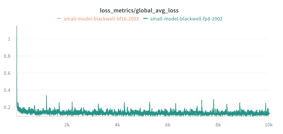
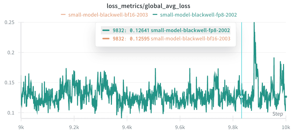
To match the training quality of BF16, we ran a series of low-precision experiments, measuring how much each recipe diverged from BF16. From these, we identified the one that yields training loss convergence nearly identical to that of BF16 for our workloads.
Specifically, we use the MXFP8 format with FP8E4M3 (4 exponent bits, 3 mantissa bits) as the element data type, FPE8M0 (8 exponent bits) as the scale data type, and a scaling block size of 32. We also adopt the MXFP8 quantization recipe from the paper, “Recipes for Pre-training LLMs with MXFP8”. Let:
-
BF16 (or FP32) vector
-
Corresponding FP8E4M3 vector
-
FP8E8M0 scale S
We calculate Q and S as follows:
where cast_to_fp8e8m0 rounds up to the nearest powers of 2 and min-clamps to , and cast_to_fp8e4m3 saturates out-of-range values and rounds to nearest, ties to even.
With this, our FP8 training loss matched the BF16 training loss:
Embracing tcgen05 MXFP8 block-scaled matrix multiplication
On the NVIDIA Blackwell architecture, MX formats are baked into the tensor cores. Block scaling is invoked through the tcgen05.mma...block_scale instruction and handled in hardware. This eliminates the need to move data out of TMEM for dequantization, since everything occurs during the tensor core matrix multiplication. Our MXFP8 matrix multiplication kernel design must therefore revolve around tcgen05.mma and operate within its constraints to achieve maximum performance.
There are several important considerations. First, the tcgen05.mma instruction requires only a single thread to launch asynchronously. This contrasts with Hopper, where the wgmma instruction needs an entire warpgroup (128 threads) to launch asynchronously. Consequently, we have to deviate from the producer-consumer pattern common in Hopper kernels, where 256+ threads are dedicated to launching matrix multiplications.
Second, tcgen05.mma supports 2-CTA matrix multiplication, where two SMs collaboratively execute a matrix multiplication by sharing the B matrix. This reduces both memory traffic and shared memory usage, allowing for a deeper matrix multiplication pipeline. Our benchmarks indicate that this 2-CTA mode delivers about a 15~20% speedup for MXFP8 matrix multiplications compared to non-clustered versions, making it essential for peak performance.
Third, as noted earlier, tcgen05.mma accumulates results in TMEM rather than in registers. While this reduces register pressure, it also introduces additional data movement between TMEM and registers through the tcgen05.ld and tcgen05.st instructions. We must ensure that these data movements are minimized.
Finally, tcgen05.mma instruction requires the scale factor to reside in TMEM. However, there is no direct method to load the scales from HBM into TMEM. The fastest approach is to first load the data from HBM into on-chip SMEM using the cp.async.bulk.tensor instruction (leveraging the Tensor Memory Accelerator, or TMA), and then transfer it from SMEM to TMEM using the tcgen05.cp instruction. For this to work, scale factors must be stored in the layout expected by tcgen05.mma, as explained later in this post.
All of the instructions involved in these considerations — tcgen05.mma, cp.async.bulk.tensor, tcgen05.cp, tcgen05.ld, and tcgen05.st — are launched asynchronously by a single thread. This allows us to apply warp specialization and design a pipelined dataflow, using TMEM and SMEM as circular buffers.
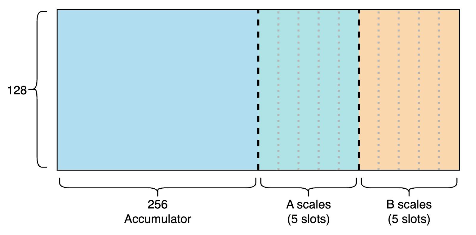
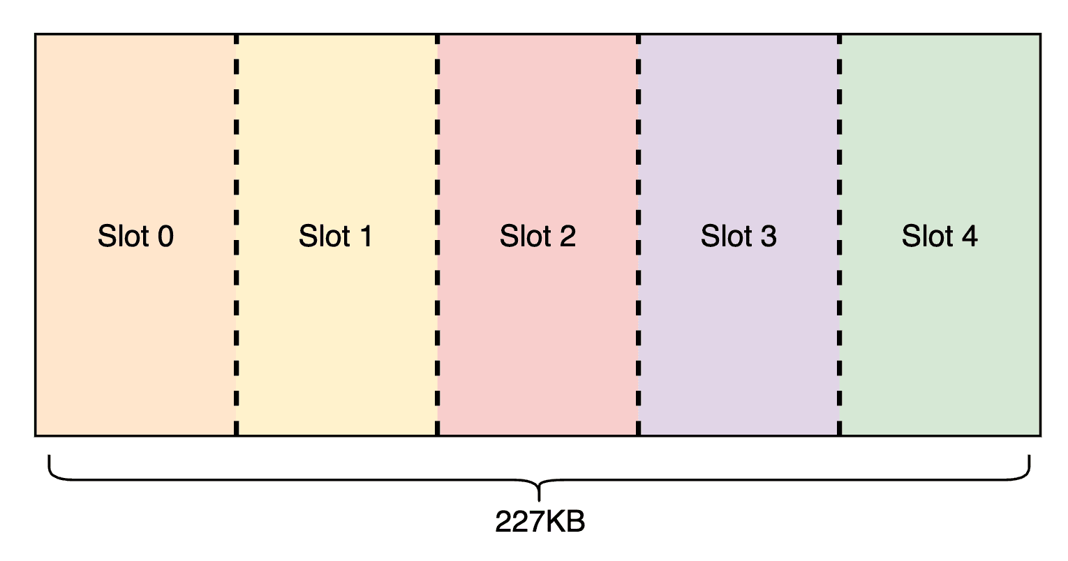
To do this, we first partition TMEM and SMEM. On Blackwell, we are given 128x512 TMEM (32-bit per cell) and 227 KB of contiguous SMEM per threadblock. We divide TMEM into 5 slots for A and B scale storage, leaving space for matrix multiplication accumulations (MMA). Similarly, in SMEM we reserve space for storing MMA results back to HBM, and partition the rest into 5 slots for loading input tiles and scale factors. The layout is illustrated below.
With this setup, we design a pipeline where certain warps continuously load input tiles and scale from HBM to SMEM, others move scales from SMEM to TMEM, others launch the MMAs, and some occasionally load the TMEM accumulator into registers, store it in SMEM, and TMA-store it back to HBM.
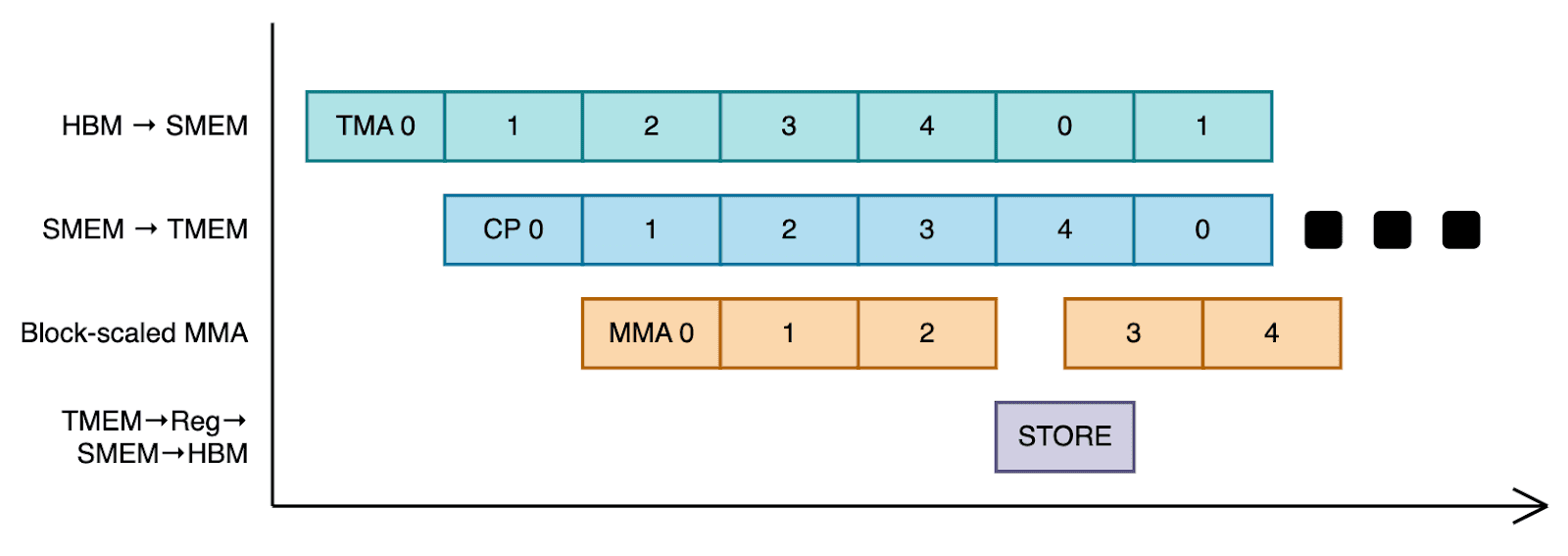
Specifically, we assign 3 warpgroups (384 threads) to each threadblock, and specialize the warpgroups into two: 2 warpgroups will only perform TMEM → register → SMEM → HBM data flow, which has the highest register pressure. The other warpgroup will do warp-specialization. Warp 0 loads the input tiles from HBM to SMEM, warp 1 loads the scale from HBM to SMEM, warp 2 loads the scale from SMEM to TMEM, and warp 3 launches the tensor core matrix multiplies. We also implement a persistent grid pattern, assigning a single threadblock per SM (148 on Blackwell GPUs) so that new input tiles can be loaded while results are being stored back to HBM.
The pseudo-code for the pipeline looks as follows:
if (warpgroup_id < 2) {
    for (int i = 0; i < num_tiles; i++) {
        mbarrier_wait_for_final_matmul_completion(); // mbarrier.try_wait
        async_load_from_TMEM(reg, TMEM); // tcgen05.ld
        wait_for_load_completion(); // tcgen05.wait
        // This is iterated in the actual implementation to save SMEM
        store_to_SMEM(SMEM, reg);
        TMA_async_store(HBM, SMEM); // cp.async.bulk.tensor
    }
} else {
    if (warp_id == 0) {
        for (int i = 0; i < num_tiles; i++) {
            for (int j = 0; j < num_iters; j++) {
                mbarrier_wait_for_matmul_completion();
                // load input tiles
                TMA_async_load(SMEM, HBM);
            }
        }
    } else if (warp_id == 1) {
        for (int i = 0; i < num_tiles; i++) {
            for (int j = 0; j < num_iters; j++) {
                mbarrier_wait_for_tcgen05_cp_completion();
                // load scales (HBM -> SMEM)
                TMA_load(SMEM, HBM);
            }
        }
    } else if (warp_id == 2) {
        for (int i = 0; i < num_tiles; i++) {
            for (int j = 0; j < num_iters; j++) {
                mbarrier_wait_for_matmul_completion();
                mbarrier_wait_for_scale_SMEM_load();
                // load scales (SMEM -> TMEM)
                load_to_TMEM(TMEM, SMEM); // tcgen05.cp
            }
        }
    } else if (cta_rank == 0) { // 2-CTA MMA is launched by a single CTA
        for (int i = 0; i < num_tiles; i++) {
            mbarrier_wait_for_TMEM_clear();
            for (int j = 0; j < num_iters; j++) {
                mbarrier_wait_for_input_SMEM_load();
                mbarrier_wait_for_scale_TMEM_load();
                // tcgen05.mma.cta_group::2.mxf8f6f4.block_scale
                launch_matmul(SMEM, SMEM, TMEM);
            }
        }
    }
}
One unavoidable limitation in block-scaled matrix multiplication on Blackwell GPUs is the size of TMEM. Our microbenchmarks show that Blackwell tensor cores achieve the highest throughput when the full 128x512 TMEM is used as the accumulator. For 2-CTA FP8 matrix multiplication, this corresponds to consistently running two 256x32x256 tcgen05.mma instructions. Each tcgen05.mma consumes a 128x256 region of TMEM per CTA, so two of them together fully occupy the 128x512 TMEM arrays across both CTAs.
When scale factors must also reside in TMEM, however, we can only execute a single 256x32x256 tcgen05.mma instruction at a time using just a 128x256 region of TMEM. As a result, performance degradation is unavoidable. For example, the throughput of a 16,384x16,384x16,384 FP8 matrix multiplication drops from 3,200 TFLOP/s to 3,040 TFLOP/s under this constraint.
These throughput numbers apply only to pure FP8 matrix multiplication. With MXFP8 block scaling, throughput inevitably decreases further due to TMEM pipelining overhead. In practice, we achieve around 2,750 TFLOP/s with L2 cache clearance for block-scaled MXFP8 matrix multiplication kernels. Even so, this remains ~1.83x faster than standard BF16 matrix multiplication, which typically reaches 1,500~1,550 TFLOP/s on optimal shapes. Not too bad of a start!
Expanding to MXFP8 grouped matrix multiplications
A standalone MXFP8 matrix multiplication kernel is a useful first step, but during MXFP8 MoE training, its applications are limited (e.g., shared expert scenarios). To fully support MoE in MXFP8, we need grouped matrix multiplication kernels, specifically:
-
Grouped forward propagation (Fprop) / data gradient (Dgrad)
-
Grouped weight gradient (Wgrad)
Note that these variants are part of the reason we are building these kernels from scratch. To date, we have not found any open-source alternative that fully supports MXFP8 MoE training with 32-block scaling.
At the kernel level, grouped Fprop and Dgrad share the same structure. The only difference is that Dgrad requires accumulation, since the input tensor passes through both the up and gate projections. But this can be easily implemented by replacing the cp.async.bulk.tensor instruction with cp.reduce.async.bulk.tensor, which can perform atomic add-store to HBM asynchronously.
Given the following matrices:
-
A:
num_tokensxin_dim -
W:
Exin_dimxout_dim, whereEis the number of experts on the current rank -
O:
num_tokensxout_dim
and assuming tokens are ordered by expert index, the grouped Fprop/Dgrad kernel performs:
for i in range(num_routed_experts):
    start = 0 if i == 0 else end
    end = start + assigned_tokens_per_expert[i]
    O[start:end, :] = A[start:end, :] @ W[i, :, :]
Grouped Wgrad, on the other hand, differs in that expert division occurs along the K (reduction) axis rather than the M axis. It computes:
for i in range(num_routed_experts):
    start = 0 if i == 0 else end
    end = start + assigned_tokens_per_expert[i]
W_grad[i, :, :] = A.T[:, start:end] @ O[start:end, :]Kernel abstraction
At the kernel level, the common unit of work is a matrix multiply-accumulate over a specified row, column, and reduction range. Abstracting this unit proved highly useful for implementing grouped matrix multiplication kernels and allowed us to reuse the original MXFP8 matrix multiplication kernel with minimal changes. Accordingly, we factored out the original kernel:
// All units of 128
int expert_idx = ... // 0 for 2D case
int row_block_idx = ...
int col_block_idx = ...
int reduction_block_start_idx = ...
int reduction_block_end_idx = ...

// Based on MXFP8 matrix multiplication implemented above
// Runs at 256x128 granularity when possible (if not, 128x128)
run_mxfp8_matmul(
    expert_idx,
    row_block_idx,
    col_block_idx,
    reduction_block_start_idx,
    reduction_block_end_idx
);
With this abstraction, implementing the grouped MXFP8 matrix multiplication variants reduces to designing the appropriate loop structures and assigning indices correctly before launching the above abstraction. However, naive looping can significantly hurt performance due to poor L2 cache utilization.
L2 cache optimization via expert-wise supergrouping
Maintaining high L2 cache utilization is critical. In our benchmarks, inefficient HBM access patterns could reduce performance by nearly 50% in grouped matrix multiplication kernels. To address this, we applied supergrouping, a heuristic from ThunderKittens kernels that maximizes L2 reuse by ensuring that the region of the output matrix computed by all 148 SMs at any given time is as square as possible. You can learn more about this by reading the linked kernel code above.
A key enhancement for our grouped matrix multiplication kernels was applying supergrouping per expert, considering only the submatrix belonging to the current expert rather than the entire output matrix. This proved especially effective for grouped Wgrad, where the reduction axis is often narrow due to expert partitioning. A narrow reduction axis leads to lower tensor core utilization, making memory bandwidth the primary bottleneck.
With the right matrix multiplication kernel abstraction and expert-wise L2 cache optimization, we achieved ~2,650 TFLOP/s with grouped MXFP8 matrix multiplication kernels — only a 4% drop compared to the non-grouped version. Great!
Grouped matrix multiplication benchmarks
The closest open-source alternative on Blackwell for grouped Fprop/Dgrad/Wgrad is DeepSeek’s DeepGEMM. DeepGEMM differs slightly in that it uses 1x128 and 128x128 scale blocks for the A and B matrices, which comes at the cost of reduced accuracy. Still, it is the only alternative available, so we integrated DeepGEMM into our internal model training and profiled its performance. While DeepGEMM excelled on certain input shapes in our microbenchmarks, our end-to-end benchmarks showed that our kernels outperformed it for our workloads.
| DeepSeek DeepGEMM | Ours | |
|---|---|---|
| Grouped Fprop / Dgrad | 0.67 ms | 0.43 ms |
| Grouped Wgrad | 0.71 ms | 0.65 ms |
Table 3. Average latency for grouped Fprop/Dgrad and Wgrad kernels during internal model training.
It is also important to note that the above benchmarks exclude quantization time. DeepGEMM does not provide optimized quantization kernels, and without them, end-to-end performance can quickly degrade. In the worst case, it can even be slower than BF16 training.
Building the fastest MXFP8 quantization kernel ever
As noted earlier, existing MXFP8 quantization kernels are not only suboptimal but also require reshaping to match tcgen05.mma scale factor layout, incurring extra runtime overhead. Our goal, therefore, was to design a quantization kernel that:
-
Fully saturates memory bandwidth, preferably exceeding 6 TB/s for large M-dimension shapes.
-
Produces the scale matrix in the exact layout expected by
tcgen05.mma, allowing our MXFP8 kernel to execute HBM → SMEM → TMEM data flow without intermediate transformations.
It turned out there was no single “magic” design that instantly gave us peak performance; it was a combination of the right primitives and numerous micro-optimizations discovered through trial and error. The most significant wins came from removing TMA swizzling in favor of a manual swizzling pattern to reduce intra-warp overhead, relying on the warp scheduler and inter-threadblock asynchrony rather than manual intra-threadblock overlapping, and minimizing SMEM and register usage to increase SM occupancy. Then there are all the standard optimizations including the TMAs, eliminating SMEM bank conflicts, leveraging fast vector intrinsics, etc. But there really isn’t much to generalize.
With these optimizations, we implemented an MXFP8 quantization kernel that sustains 6.2+ TB/s while producing the scale matrix in a layout directly compatible with tcgen05.mma. To the best of our knowledge, this is the fastest MXFP8 quantization kernel available for MoE training.
| NVIDIA TransformerEngine | PyTorch TorchAO | Ours | |
|---|---|---|---|
| Naive | 5236.35 GB/s | 5245.15 GB/s | Not applicable |
| With reshape | 4430.27 GB/s | 4524.45 GB/s | 6212.21 GB/s |
Table 4. MXFP8 quantization kernel comparison (E4M3, 32-block scaling) by memory bandwidth utilization. "With reshape" includes the time to reshape the scale factor for tcgen05.mma.
Other optimizations to the MXFP8 quantization included building a fused quantization kernel that outputs both non-transposed and transposed results (the latter needed for backward passes), as well as fusing MXFP8 quantization logic directly into other kernels to minimize HBM access as much as possible. For example, we attached MXFP8 dequantization/quantization logic to the prologue and epilogue of our fused MXFP8 SwiGLU kernel.
Speedups!
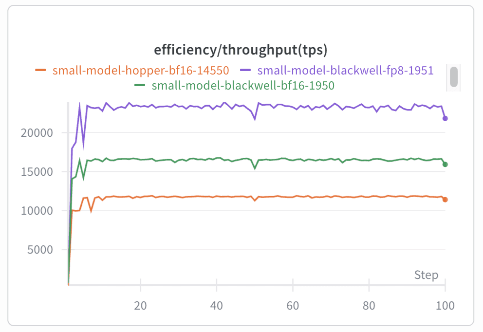
With all the optimizations described above, we achieved 3.5x faster MoE layer execution for both the forward and backward passes while maintaining the same training quality. When tested on one of our internal models, this translated into a 1.5x end-to-end training speedup on Blackwell and a 2x speedup compared to our original Hopper setup, measured in tokens per second per GPU (TPS/GPU). We believe that our stack runs MXFP8 MoE training faster than any combination of open-source alternatives.
| Hopper BF16 | Blackwell BF16 | Blackwell MXFP8 | |
|---|---|---|---|
| MoE Forward (ms) | 32.36 ms | 25.96 ms | 9.45 ms |
| MoE Backward (ms) | 63.24 ms | 59.17 ms | 17.04 ms |
| End-to-end (TPS/GPU) | 12k TPS/GPU | 16k TPS/GPU | 24k TPS/GPU |
Table 5. Performance comparisons (internal model). Note: Blackwell BF16 MoE was a direct port of the Hopper code
Closing thoughts
We still have plenty of work ahead and many kernels left to optimize. Our current efforts focus on building more efficient multi-GPU communication, improving custom attention kernels, and preparing to transition to FP4 for future MoE training runs.
If you are interested in writing and optimizing high-performance kernels, training large coding models, or our work broadly, we’d love to hear from you. Reach out to us at hiring@cursor.com.
Special thanks to Benjamin Spector, Sasha Rush, Less Wright, Federico Cassano, Rohan Shah, Jacob Jackson, Sujay Jayakar, and Shengtong Zhang for reading this post and offering valuable feedback.